DATA SCIENCE NOTES -Introduction to AI and ML (MINOR)

What is Data Science?

Data Science is the process of extracting and analysing useful information from data to solve problems that are difficult to solve analytically. For example, when you visit an e-commerce site and look at a few categories and products before making a purchase, you are creating data that Analysts can use to figure out how you make purchases.

It involves different disciplines like mathematical and statistical modelling, extracting data from its source and applying data visualization techniques. It also involves handling big data technologies to gather both structured and unstructured data.

Data Science is an interdisciplinary field that uses:

Statistics
Programming
Machine Learning
Domain Knowledge

to extract useful insights and knowledge from data.

2. Why Data Science is Important?

Because data is everywhere:

Social Media (likes, comments)
Healthcare (patient records)
Banking (transactions)
Education (student performance)
E-commerce (recommendations)

📊 Companies use Data Science to:

Predict sales
Detect fraud
Recommend products
Improve services

3. Types of Data

a) Structured Data

Tables, rows, columns
Example: Excel sheet of student marks

Roll No	Name	Marks
1	A	78

b) Unstructured Data

Images, videos, text, audio
Example: YouTube videos, tweets

c) Semi-Structured Data

JSON, XML
Example: API responses

4. Data Science Life Cycle

Problem Definition
Data Collection
Data Cleaning
Exploratory Data Analysis (EDA)
Model Building
Evaluation
Deployment

📌 Example:
Predicting student performance using attendance and marks.

5. Tools Used in Data Science

Programming: Python, R
Libraries: NumPy, Pandas, Matplotlib, Scikit-learn
Databases: MySQL, MongoDB
Visualization: Power BI, Tableau

INTRODUCTION TO MACHINE LEARNING AND AI

Machine learning (ML) is a type of algorithm that lets software get more accurate at predicting what will happen in future without being specifically programmed to do so. The basic idea behind machine learning is to make algorithms that can take data as input and use statistical analysis to predict an output while also updating outputs as new data becomes available.
Machine learning is a part of artificial intelligence that uses algorithms to find patterns in data and then predict how those patterns will change in the future. This lets engineers use statistical analysis to look for patterns in the data.
Facebook, Twitter, Instagram, YouTube, and TikTok collect information about their users, based on what you've done in the past, it can guess your interests and requirements and suggest products, services, or articles that fit your needs.
Machine learning is a set of tools and concepts that are used in data science, but they also show up in other fields. Data scientists often use machine learning in their work to help them get more information faster or figure out trends.

Types of Machine Learning
Machine learning can be classified into three types of algorithms −
Supervised learning
Unsupervised learning
Reinforcement learning
Supervised Learning
Supervised learning is a type of machine learning and artificial intelligence. It is also called "supervised machine learning." It is defined by the fact that it uses labelled datasets to train algorithms how to correctly classify data or predict outcomes. As data is put into the model, its weights are changed until the model fits correctly. This is part of the cross validation process. Supervised learning helps organisations find large-scale solutions to a wide range of real-world problems, like classifying spam in a separate folder from your inbox like in Gmail we have a spam folder.
Supervised Learning Algorithms
Some supervised learning algorithms are −
Naive Bayes − Naive Bayes is a classification algoritm that is based on the Bayes Theorem's principle of class conditional independence. This means that the presence of one feature doesn't change the likelihood of another feature, and that each predictor has the same effect on the result/outcome.
Linear Regression − Linear regression is used to find how a dependent variable is related to one or more independent variables and to make predictions about what will happen in the future. Simple linear regression is when there is only one independent variable and one dependent variable.
Logistic Regression − When the dependent variables are continuous, linear regression is used. When the dependent variables are categorical, like "true" or "false" or "yes" or "no," logistic regression is used. Both linear and logistic regression seek to figure out the relationships between the data inputs. However, logistic regression is mostly used to solve binary classification problems, like figuring out if a particular mail is a spam or not.
Support Vector Machines(SVM) − A support vector machine is a popular model for supervised learning developed by Vladimir Vapnik. It can be used to both classify and predict data. So, it is usually used to solve classification problems by making a hyperplane where the distance between two groups of data points is the greatest. This line is called the "decision boundary" because it divides the groups of data points (for example, oranges and apples) on either side of the plane.
K-nearest Neighbour − The KNN algorithm, which is also called the "k-nearest neighbour" algorithm, groups data points based on how close they are to and related to other data points. This algorithm works on the idea that data points that are similar can be found close to each other. So, it tries to figure out how far apart the data points are, using Euclidean distance and then assigns a category based on the most common or average category. However, as the size of the test dataset grows, the processing time increases, making it less useful for classification tasks.
Random Forest − Random forest is another supervised machine learning algorithm that is flexible and can be used for both classification and regression. The "forest" is a group of decision trees that are not correlated to each other. These trees are then combined to reduce variation and make more accurate data predictions.
Unsupervised Learning
Unsupervised learning, also called unsupervised machine learning, uses machine learning algorithms to look at unlabelled datasets and group them together. These programmes find hidden patterns or groups of data. Its ability to find similarities and differences in information makes it perfect for exploratory data analysis, cross-selling strategies, customer segmentation, and image recognition.
Common Unsupervised Learning Approaches
Unsupervised learning models are used for three main tasks: clustering, making connections, and reducing the number of dimensions. Below, we'll describe learning methods and common algorithms used −
Clustering − Clustering is a method for data mining that organises unlabelled data based on their similarities or differences. Clustering techniques are used to organise unclassified, unprocessed data items into groups according to structures or patterns in the data. There are many types of clustering algorithms, including exclusive, overlapping, hierarchical, and probabilistic.
K-means Clustering is a popular example of an clustering approach in which data points are allocated to K groups based on their distance from each group's centroid. The data points closest to a certain centroid will be grouped into the same category. A higher K number indicates smaller groups with more granularity, while a lower K value indicates bigger groupings with less granularity. Common applications of K-means clustering include market segmentation, document clustering, picture segmentation, and image compression.
Dimensionality Reduction − Although more data typically produces more accurate findings, it may also affect the effectiveness of machine learning algorithms (e.g., overfitting) and make it difficult to visualize datasets. Dimensionality reduction is a strategy used when a dataset has an excessive number of characteristics or dimensions. It decreases the quantity of data inputs to a manageable level while retaining the integrity of the dataset to the greatest extent feasible. Dimensionality reduction is often employed in the data pre-processing phase, and there are a number of approaches, one of them is −
Principal Component Analysis (PCA) − It is a dimensionality reduction approach used to remove redundancy and compress datasets through feature extraction. This approach employs a linear transformation to generate a new data representation, resulting in a collection of "principal components." The first principal component is the dataset direction that maximises variance. Although the second principal component similarly finds the largest variance in the data, it is fully uncorrelated with the first, resulting in a direction that is orthogonal to the first. This procedure is repeated dependent on the number of dimensions, with the next main component being the direction orthogonal to the most variable preceding components.
Reinforcement Learning
Reinforcement Learning (RL) is a type of machine learning that allows an agent to learn in an interactive setting via trial and error utilising feedback from its own actions and experiences.
Key terms in Reinforcement Learning
Some significant concepts describing the fundamental components of an RL issue are −
Environment − The physical surroundings in which an agent functions
Condition − The current standing of the agent
Reward − Environment-based feed-back
Policy − Mapping between agent state and actions
Value − The future compensation an agent would obtain for doing an action in a given condition.
Data Science vs Machine Learning
Data Science is the study of data and how to derive meaningful insights from it, while machine learning is the study and development of models that use data to enhance performance or inform predictions. Machine learning is a subfield of artificial intelligence.
In recent years, machine learning and artificial intelligence (AI) have come to dominate portions of data science, playing a crucial role in data analytics and business intelligence. Machine learning automates data analysis and makes predictions based on the collection and analysis of massive volumes of data about certain populations using models and algorithms. Data Science and machine learning are related to each other, but not identical.
Data Science is a vast field that incorporates all aspects of deriving insights and information from data. It involves gathering, cleaning, analysing, and interpreting vast amount of data to discover patterns, trends, and insights that may guide business choices.
Machine learning is a subfield of data science that focuses on the development of algorithms that can learn from data and make predictions or judgements based on their acquired knowledge. Machine learning algorithms are meant to enhance their performance automatically over time by acquiring new knowledge.
In other words, data science encompasses machine learning as one of its numerous methodologies. Machine learning is a strong tool for data analysis and prediction, but it is just a subfield of data science as a whole.
Given below is the table of comparison for a clear understanding.
Data Science Machine Learning
Data Science is a broad field that involves the extraction of insights and knowledge from large and complex datasets using various techniques, including statistical analysis, machine learning, and data visualization.
Machine learning is a subset of data science that involves defining and developing algorithms and models that enable machines to learn from data and make predictions or decisions without being explicitly programmed.
Data Science focuses on understanding the data, identifying patterns and trends, and extracting insights to support decision-making.
Machine learning, on the other hand, focuses on building predictive models and making decisions based on the learned patterns.
Data Science includes a wide range of techniques, such as data cleaning, data integration, data exploration, statistical analysis, data visualization, and machine learning.
Machine learning, on the other hand, primarily focuses on building predictive models using algorithms such as regression, classification, and clustering.
Data Science typically requires large and complex datasets that require significant processing and cleaning to derive insights.
Machine learning, on the other hand, requires labelled data that can be used to train algorithms and models.
Data Science requires skills in statistics, programming, and data visualization, as well as domain knowledge in the area being studied.
Machine learning requires a strong understanding of algorithms, programming, and mathematics, as well as a knowledge of the specific application area.
Data Science techniques can be used for a variety of purposes beyond prediction, such as clustering, anomaly detection, and data visualization
Machine learning algorithms are primarily focused on making predictions or decisions based on data
Data Science often relies on statistical methods to analyze data,
Machine learning relies on algorithms to make predictions or decisions.

Data Science	Machine Learning
Data Science is a broad field that involves the extraction of insights and knowledge from large and complex datasets using various techniques, including statistical analysis, machine learning, and data visualization.	Machine learning is a subset of data science that involves defining and developing algorithms and models that enable machines to learn from data and make predictions or decisions without being explicitly programmed.
Data Science focuses on understanding the data, identifying patterns and trends, and extracting insights to support decision-making.	Machine learning, on the other hand, focuses on building predictive models and making decisions based on the learned patterns.
Data Science includes a wide range of techniques, such as data cleaning, data integration, data exploration, statistical analysis, data visualization, and machine learning.	Machine learning, on the other hand, primarily focuses on building predictive models using algorithms such as regression, classification, and clustering.
Data Science typically requires large and complex datasets that require significant processing and cleaning to derive insights.	Machine learning, on the other hand, requires labelled data that can be used to train algorithms and models.
Data Science requires skills in statistics, programming, and data visualization, as well as domain knowledge in the area being studied.	Machine learning requires a strong understanding of algorithms, programming, and mathematics, as well as a knowledge of the specific application area.
Data Science techniques can be used for a variety of purposes beyond prediction, such as clustering, anomaly detection, and data visualization	Machine learning algorithms are primarily focused on making predictions or decisions based on data
Data Science often relies on statistical methods to analyze data,	Machine learning relies on algorithms to make predictions or decisions.

INTRODUCTION TO ARTIFICIAL INTELLIGENCE (AI)

1. What is Artificial Intelligence?

Artificial Intelligence (AI) is a branch of computer science that focuses on creating intelligent machines that can think, learn, and make decisions like humans.

📌 Simple Definition (for students):

Artificial Intelligence is the ability of a computer or machine to perform tasks that normally require human intelligence.

2. Why Do We Need AI?

AI helps us to:

Reduce human effort
Work faster and accurately
Solve complex problems
Make better decisions

📌 Example:

Google Maps finds the shortest route
Mobile face unlock
Chatbots answering questions

3. Examples of AI in Daily Life

Area	AI Example
Mobile Phones	Face recognition
Education	Online exam evaluation
Healthcare	Disease prediction
Banking	Fraud detection
Social Media	Friend suggestions
E-commerce	Product recommendations

4. History of Artificial Intelligence (Brief)

1950 – Alan Turing proposed “Can machines think?”
1956 – Term “Artificial Intelligence” coined by John McCarthy
1997 – IBM Deep Blue defeated chess champion
Present – AI in self-driving cars, chatbots, healthcare

5. Types of Artificial Intelligence

1. Narrow AI (Weak AI)

Performs one specific task
Example:
- Siri
- Alexa
- Google Assistant

2. General AI (Strong AI)

Can perform any intellectual task like humans
Example:
- Does not exist yet

3. Super AI

Smarter than humans
Still theoretical

6. Components of AI

Data – Information to learn from
Algorithms – Set of rules
Computing Power – Speed & memory
Learning Models – ML, DL

7. How Does AI Work? (Simple Flow)


Input Data → Learning Algorithm → Model → Prediction / Decision

📌 Example:
Photos → Face recognition algorithm → Identify person

8. AI vs Human Intelligence

Human	AI
Emotional	No emotions
Learns from experience	Learns from data
Creative	Limited creativity
Gets tired	Works 24×7

9. Subfields of Artificial Intelligence

a) Machine Learning (ML)

Machine learns from data
Example: Marks prediction

b) Deep Learning (DL)

Uses neural networks
Example: Image recognition

c) Natural Language Processing (NLP)

Understands human language
Example: Chatbots

d) Computer Vision

Understands images/videos
Example: Face detection

10. Applications of AI

Self-driving cars
Medical diagnosis
Voice assistants
Smart classrooms
Robotics
Recommendation systems

11. Advantages of AI

✔ Fast decision making
✔ Reduces errors
✔ Works continuously
✔ Handles large data

12. Disadvantages of AI

✖ Expensive
✖ Job displacement
✖ No emotions
✖ Data dependency

13. Future of AI

Smart robots
Personalized education
Advanced healthcare
Ethical AI development

14. Simple Exam Answer

Artificial Intelligence is a field of computer science that enables machines to perform tasks that require human intelligence such as learning, reasoning, and decision making. AI is widely used in healthcare, education, banking, and transportation. It helps in faster processing, accuracy, and automation.

LINEAR REGRESSION

1. What is Linear Regression? (Basic Facts)

Linear Regression is a supervised machine learning algorithm used to predict continuous numerical values by finding a linear relationship between input and output variables.

📌 Definition (Exam-Ready):

Linear Regression is a statistical and machine learning technique that models the relationship between a dependent variable and one or more independent variables using a straight line.

2. Why is it Called “Linear”?

Because the relationship between variables is represented by a straight line.

Mathematical Equation:

y = mx + c

Where:

y → dependent variable (output)
x → independent variable (input)
m → slope (rate of change)
c → intercept (value of y when x = 0)

3. Types of Linear Regression

1. Simple Linear Regression

One input variable
Example: Study Hours → Marks

y = mx + c

2. Multiple Linear Regression

More than one input variable
Example: House Price depends on area, rooms, location

y = b_0 + b_1x_1 + b_2x_2 + b_3x_3

4. Diagram: Linear Regression Concept


Marks (Y)
  |
  |            *
  |         *
  |      *
  |   *
  | *
  ----------------------------> Study Hours (X)
         Best Fit Line

Dots → actual data
Line → predicted relationship

5. Assumptions of Linear Regression

Linear relationship exists
Errors are normally distributed
No multicollinearity
Homoscedasticity (constant variance)
Independent observations

📌 Important for theory questions

6. Applications of Linear Regression

Salary prediction
Sales forecasting
Stock trend analysis
Weather prediction
Student performance analysis

IMPLEMENTATION OF LINEAR REGRESSION

7. Steps Involved in Linear Regression

Flow Diagram


Dataset
   ↓
Separate X and Y
   ↓
Train Model
   ↓
Test Model
   ↓
Prediction
   ↓
Evaluation

8. Case Study 1: Study Hours vs Marks

Dataset

Study Hours (X)	Marks (Y)
1	20
2	35
3	50
4	65
5	80

Step 1: Import Libraries


import pandas as pd
import matplotlib.pyplot as plt
from sklearn.linear_model import LinearRegression

Step 2: Create Dataset


data = {
    'Hours': [1, 2, 3, 4, 5],
    'Marks': [20, 35, 50, 65, 80]
}

df = pd.DataFrame(data)

Step 3: Separate Input and Output


X = df[['Hours']]
y = df['Marks']

Step 4: Train the Model


model = LinearRegression()
model.fit(X, y)

📌 The model learns the best fit line.

Step 5: Prediction


new_data = pd.DataFrame({'Hours': [6]})
prediction = model.predict(new_data)
print("Predicted Marks:", prediction)

Step 6: Visualization


plt.scatter(X, y)
plt.plot(X, model.predict(X))
plt.xlabel("Study Hours")
plt.ylabel("Marks")
plt.show()

Diagram Explanation


Marks
 |
 |        ●
 |     ●
 |  ●
 |●
 ------------------> Hours
     Prediction Line

9. Case Study 2: Salary Prediction

Dataset

Experience (Years)	Salary
1	15000
2	20000
3	30000
4	40000
5	50000

Implementation Code


import pandas as pd
from sklearn.linear_model import LinearRegression

data = {
    'Experience': [1, 2, 3, 4, 5],
    'Salary': [15000, 20000, 30000, 40000, 50000]
}

df = pd.DataFrame(data)

X = df[['Experience']]
y = df['Salary']

model = LinearRegression()
model.fit(X, y)

new_exp = pd.DataFrame({'Experience': [6]})
salary_pred = model.predict(new_exp)

print("Predicted Salary:", salary_pred)

10. Diagram: Experience vs Salary


Salary
 |
 |           *
 |       *
 |   *
 | *
 --------------------> Experience
       Best Fit Line

MODEL EVALUATION

11. Performance Metrics

1. Mean Squared Error (MSE)

MSE = \frac{1}{n}\sum(y - \hat{y})^2

2. Root Mean Squared Error (RMSE)

RMSE = \sqrt{MSE}

3. R² Score

Measures how well data fits the model
Value between 0 and 1

12. Advantages of Linear Regression

✔ Simple and easy to understand
✔ Fast training
✔ Interpretable results

13. Limitations of Linear Regression

✖ Works only for linear data
✖ Sensitive to outliers
✖ Poor performance for complex patterns

14. Real-World Case Studies

Case Study 3: House Price Prediction

Inputs:

Area
Bedrooms
Location

Output:

Price

Uses Multiple Linear Regression

15. Summary (For Students)

Linear Regression predicts continuous values
It draws a best-fit straight line
Simple, fast, and widely used
Works best when data is linear

16. Short Exam Answer (5 Marks)

Linear Regression is a supervised learning algorithm used for predicting continuous values. It establishes a linear relationship between independent and dependent variables using a best-fit straight line. It is widely used in salary prediction, sales forecasting, and performance analysis.

Linear regression is a type of supervised machine-learning algorithm that learns from the labelled datasets and maps the data points with most optimized linear functions which can be used for prediction on new datasets. It assumes that there is a linear relationship between the input and output, meaning the output changes at a constant rate as the input changes. This relationship is represented by a straight line.

For example we want to predict a student's exam score based on how many hours they studied. We observe that as students study more hours, their scores go up. In the example of predicting exam scores based on hours studied. Here

Independent variable (input): Hours studied because it's the factor we control or observe.
Dependent variable (output): Exam score because it depends on hobw many hours were studied.

We use the independent variable to predict the dependent variable.

Best Fit Line in Linear Regression

In linear regression, the best-fit line is the straight line that most accurately represents the relationship between the independent variable (input) and the dependent variable (output). It is the line that minimizes the difference between the actual data points and the predicted values from the model.

1. Goal of the Best-Fit Line

The goal of linear regression is to find a straight line that minimizes the error (the difference) between the observed data points and the predicted values. This line helps us predict the dependent variable for new, unseen data.

Here Y is called a dependent or target variable and X is called an independent variable also known as the predictor of Y. There are many types of functions or modules that can be used for regression. A linear function is the simplest type of function. Here, X may be a single feature or multiple features representing the problem.

2. Equation of the Best-Fit Line

For simple linear regression (with one independent variable), the best-fit line is represented by the equation

$y = m x + b$

Where:

y is the predicted value (dependent variable)
x is the input (independent variable)
m is the slope of the line (how much y changes when x changes)
b is the intercept (the value of y when x = 0)

The best-fit line will be the one that optimizes the values of m (slope) and b (intercept) so that the predicted y values are as close as possible to the actual data points.

3. Minimizing the Error: The Least Squares Method

To find the best-fit line, we use a method called Least Squares. The idea behind this method is to minimize the sum of squared differences between the actual values (data points) and the predicted values from the line. These differences are called residuals.

The formula for residuals is:

$R e s i d u a l = y ᵢ - \hat{y} ᵢ$

Where:

$y ᵢ$ is the actual observed value
$\hat{y} ᵢ$ is the predicted value from the line for that $x ᵢ$

The least squares method minimizes the sum of the squared residuals:

$S u m o f s q u a r e d e r r o r s (S S E) = Σ (y ᵢ - \hat{y} ᵢ) ²$

This method ensures that the line best represents the data where the sum of the squared differences between the predicted values and actual values is as small as possible.

4. Interpretation of the Best-Fit Line

Slope (m): The slope of the best-fit line indicates how much the dependent variable (y) changes with each unit change in the independent variable (x). For example if the slope is 5, it means that for every 1-unit increase in x, the value of y increases by 5 units.
Intercept (b): The intercept represents the predicted value of y when x = 0. It’s the point where the line crosses the y-axis.

In linear regression some hypothesis are made to ensure reliability of the model's results.

Limitations
Assumes Linearity: The method assumes the relationship between the variables is linear. If the relationship is non-linear, linear regression might not work well.
Sensitivity to Outliers: Outliers can significantly affect the slope and intercept, skewing the best-fit line.

Hypothesis function in Linear Regression

In linear regression, the hypothesis function is the equation used to make predictions about the dependent variable based on the independent variables. It represents the relationship between the input features and the target output.

For a simple case with one independent variable, the hypothesis function is:

$h (x) = β ₀ + β ₁ x$

Where:

$h (x) (o r \hat{y})$ is the predicted value of the dependent variable (y).
x $x$ is the independent variable.
$β ₀$ is the intercept, representing the value of y when x is 0.
$β ₁$ is the slope, indicating how much y changes for each unit change in x.

For multiple linear regression (with more than one independent variable), the hypothesis function expands to:

$h (x ₁, x ₂, . . ., x ₖ) = β ₀ + β ₁ x ₁ + β ₂ x ₂ + . . . + β ₖ x ₖ$

Where:

$x ₁, x ₂, . . ., x ₖ$ are the independent variables.
$β ₀$ is the intercept.
$β ₁, β ₂, . . ., β ₖ$ are the coefficients, representing the influence of each respective independent variable on the predicted output.

Assumptions of the Linear Regression

1. Linearity: The relationship between inputs (X) and the output (Y) is a straight line.

2. Independence of Errors: The errors in predictions should not affect each other.

3. Constant Variance (Homoscedasticity): The errors should have equal spread across all values of the input. If the spread changes (like fans out or shrinks), it's called heteroscedasticity and it's a problem for the model.

4. Normality of Errors: The errors should follow a normal (bell-shaped) distribution.

5. No Multicollinearity(for multiple regression): Input variables shouldn’t be too closely related to each other.

6. No Autocorrelation: Errors shouldn't show repeating patterns, especially in time-based data.

7. Additivity: The total effect on Y is just the sum of effects from each X, no mixing or interaction between them.'

To understand Multicollinearity detail refer to article: Multicollinearity.

Types of Linear Regression

When there is only one independent feature it is known as Simple Linear Regression or Univariate Linear Regression and when there are more than one feature it is known as Multiple Linear Regression or Multivariate Regression.

1. Simple Linear Regression

Simple linear regression is used when we want to predict a target value (dependent variable) using only one input feature (independent variable). It assumes a straight-line relationship between the two.

Formula

$\hat{y} = θ_{0} + θ_{1} x$

Where:

$\hat{y}$ is the predicted value
$x$ is the input (independent variable)
$θ_{0}$ is the intercept (value of $\hat{y} $ when x=0)
$θ_{1}$ is the slope or coefficient (how much $\hat{y}$ changes with one unit of x)

Example:

Predicting a person’s salary (y) based on their years of experience (x).

2. Multiple Linear Regression

Multiple linear regression involves more than one independent variable and one dependent variable. The equation for multiple linear regression is:

$\hat{y} = θ_{0} + θ_{1} x_{1} + θ_{2} x_{2} + \dots + θ_{n} x_{n}$

where:

$\hat{y}$ is the predicted value
$x_{1}, x_{2}, \dots, x_{n}$ are the independent variables
$θ_{1}, θ_{2}, \dots, θ_{n}$ are the coefficients (weights) corresponding to each predictor.
$θ_{0}$ is the intercept.

The goal is to find the best-fit line that predicts Y accurately for given inputs X.

Use Cases

Real Estate: Predict property prices using location, size and other factors.
Finance: Forecast stock prices using interest rates and inflation data.
Agriculture: Estimate crop yield from rainfall, temperature and soil quality.
E-commerce: Analyze how price, promotions and seasons affect sales.

Once you understand linear regression and its types, the next step is building the model in practice.

Cost function for Linear Regression

In Linear Regression, the cost function measures how far the predicted values ( $\hat{Y}$ ) are from the actual values (Y). It helps identify and reduce errors to find the best-fit line. The most common cost function used is Mean Squared Error (MSE), which calculates the average of squared differences between actual and predicted values:

$Cost function (J) = \frac{1}{n} \sum_{n}^{i} (\hat{y_{i}} - y_{i})^{2}$

Here, $\hat{y_{i}} = θ_{1} + θ_{2} x_{i}$

To minimize this cost, we use Gradient Descent, which iteratively updates θ1 and θ2 until the MSE reaches its lowest value. This ensures the line fits the data as accurately as possible.

Gradient Descent for Linear Regression

Gradient descent is an optimization technique used to train a linear regression model by minimizing the prediction error. It works by starting with random model parameters and repeatedly adjusting them to reduce the difference between predicted and actual values.

How it works:

Start with random values for slope and intercept.
Calculate the error between predicted and actual values.
Find how much each parameter contributes to the error (gradient).
Update the parameters in the direction that reduces the error.
Repeat until the error is as small as possible.

This helps the model find the best-fit line for the data.

For more details you can refer to: Gradient Descent in Linear Regression

Evaluation Metrics for Linear Regression

A variety of evaluation measures can be used to determine the strength of any linear regression model. These assessment metrics often give an indication of how well the model is producing the observed outputs.

The most common measurements are:

1. Mean Square Error (MSE)

Mean Squared Error (MSE) is an evaluation metric that calculates the average of the squared differences between the actual and predicted values for all the data points. The difference is squared to ensure that negative and positive differences don't cancel each other out.

$M S E = \frac{1}{n} \sum_{i = 1}^{n} {(y_{i} - \hat{y_{i}})}^{2}$

Here,

$n$ is the number of data points.
$y_{i}$ is the actual or observed value for the $i^{t h}$ data point.
$\hat{y_{i}}$ is the predicted value for the $i^{t h}$ data point.

MSE is a way to quantify the accuracy of a model's predictions. MSE is sensitive to outliers as large errors contribute significantly to the overall score.

2. Mean Absolute Error (MAE)

Mean Absolute Error is an evaluation metric used to calculate the accuracy of a regression model. MAE measures the average absolute difference between the predicted values and actual values.

Mathematically MAE is expressed as:

$M A E = \frac{1}{n} \sum_{i = 1}^{n} ∣ Y_{i} - \hat{Y_{i}} ∣$

Here,

n is the number of observations
Yi represents the actual values.
$\hat{Y_{i}}$ represents the predicted values

Lower MAE value indicates better model performance. It is not sensitive to the outliers as we consider absolute differences.

3. Root Mean Squared Error (RMSE)

The square root of the residuals' variance is the Root Mean Squared Error. It describes how well the observed data points match the expected values or the model's absolute fit to the data. In mathematical notation, it can be expressed as:

$R M S E = \sqrt{\frac{R S S}{n}} = \sqrt{\frac{\sum_{i = 2}^{n} (y_{i}^{a c t u a l} - y_{i}^{p r e d i c t e d})^{2}}{n}}$

Where:

$n$ : Number of observations
$y_{i}$ : Actual value
$\hat{y_{i}}$ : Predicted value

RMSE is in the same unit as the target variable and highlights larger errors more clearly.

4. Coefficient of Determination (R-squared)

R-Squared is a statistic that indicates how much variation the developed model can explain or capture. It is always in the range of 0 to 1. In general, the better the model matches the data, the greater the R-squared number.
In mathematical notation, it can be expressed as:

$R^{2} = 1 - (^{\frac{R S S}{T S S}})$

Residual sum of Squares(RSS): The sum of squares of the residual for each data point in the plot or data is known as the residual sum of squares or RSS. It is a measurement of the difference between the output that was observed and what was anticipated.

$R S S = \sum_{i = 1}^{n} (y_{i} - b_{0} - b_{1} x_{i})^{2}$

Total Sum of Squares (TSS): The sum of the data points' errors from the answer variable's mean is known as the total sum of squares or TSS.

$T S S = \sum_{i = 1}^{n} (y - \overline{y_{i}})^{2}$ .

R squared metric is a measure of the proportion of variance in the dependent variable that is explained the independent variables in the model.

5. Adjusted R-Squared Error

Adjusted $R^{2}$ measures the proportion of variance in the dependent variable that is explained by independent variables in a regression model. Adjusted R-square accounts the number of predictors in the model and penalizes the model for including irrelevant predictors that don't contribute significantly to explain the variance in the dependent variables.

Mathematically, adjusted $R^{2}$ is expressed as:

$A d j u s t e d R^{2} = 1 - (\frac{(1 - R^{2}) . (n - 1)}{n - k - 1})$

Here,

n is the number of observations
k is the number of predictors in the model
R2 is coeeficient of determination

It penalizes the inclusion of unnecessary predictors, helping to prevent overfitting.

Regularization Techniques for Linear Models

1. Lasso Regression (L1 Regularization)

Lasso Regression is a technique used for regularizing a linear regression model, it adds a penalty term to the linear regression objective function to prevent overfitting.

The objective function after applying lasso regression is:

$J (θ) = \frac{1}{2 m} \sum_{i = 1}^{m} (\hat{y_{i}} - y_{i})^{2} + λ \sum_{j = 1}^{n} ∣ θ_{j} ∣$

the first term is the least squares loss, representing the squared difference between predicted and actual values.
the second term is the L1 regularization term, it penalizes the sum of absolute values of the regression coefficient θj.

2. Ridge Regression (L2 Regularization)

Ridge regression is a linear regression technique that adds a regularization term to the standard linear objective. Again, the goal is to prevent overfitting by penalizing large coefficient in linear regression equation. It useful when the dataset has multicollinearity where predictor variables are highly correlated.

The objective function after applying ridge regression is:

$J (θ) = \frac{1}{2 m} \sum_{i = 1}^{m} (\hat{y_{i}} - y_{i})^{2} + λ \sum_{j = 1}^{n} θ_{j}^{2}$

the first term is the least squares loss, representing the squared difference between predicted and actual values.
the second term is the L1 regularization term, it penalizes the sum of square of values of the regression coefficient θj.

3. Elastic Net Regression

Elastic Net Regression is a hybrid regularization technique that combines the power of both L1 and L2 regularization in linear regression objective.

$J (θ) = \frac{1}{2 m} \sum_{i = 1}^{m} (\hat{y_{i}} - y_{i})^{2} + α λ \sum_{j = 1}^{n} ∣ θ_{j} ∣ + \frac{1}{2} (1 - α) λ \sum_{j = 1} n θ_{j}^{2}$

the first term is least square loss.
the second term is L1 regularization and third is ridge regression.
$λ$ is the overall regularization strength.
$α$ controls the mix between L1 and L2 regularization.

Now that we have learned how to make a linear regression model, now we will implement it.

Python Implementation of Linear Regression

1. Import the necessary libraries

import numpy as np
import matplotlib.pyplot as plt
from sklearn.linear_model import LinearRegression

2. Generating Random Dataset

Fetches the California Housing dataset and separates features (X) and target (y).

np.random.seed(42)

X = np.random.rand(50, 1) * 100  

Y = 3.5 * X + np.random.randn(50, 1) * 20 

3. Creating and Training Linear Regression Model

model = LinearRegression()
model.fit(X, Y) 

4. Predicting Y Values

Y_pred = model.predict(X)

5. Visualizing the Regression Line

plt.figure(figsize=(8,6)) 
plt.scatter(X, Y, color='blue', label='Data Points') 
plt.plot(X, Y_pred, color='red', linewidth=2, label='Regression Line') 
plt.title('Linear Regression on Random Dataset')
plt.xlabel('X')
plt.ylabel('Y')
plt.legend()
plt.grid(True)
plt.show()

Output:

6. Slope and Intercept

print("Slope (Coefficient):", model.coef_[0][0])
print("Intercept:", model.intercept_[0])

Output:

Slope (Coefficient): 3.4553132007706204
Intercept: 1.9337854893777546

Why Linear Regression is Important

Here’s why linear regression is important:

Simplicity and Interpretability: It’s easy to understand and interpret, making it a starting point for learning about machine learning.
Predictive Ability: Helps predict future outcomes based on past data, making it useful in various fields like finance, healthcare and marketing.
Basis for Other Models: Many advanced algorithms, like logistic regression or neural networks, build on the concepts of linear regression.
Efficiency: It’s computationally efficient and works well for problems with a linear relationship.
Widely Used: It’s one of the most widely used techniques in both statistics and machine learning for regression tasks.
Analysis: It provides insights into relationships between variables (e.g., how much one variable influences another).

Advantages

Linear regression is a relatively simple algorithm, making it easy to understand and implement. The coefficients of the linear regression model can be interpreted as the change in the dependent variable for a one-unit change in the independent variable, providing insights into the relationships between variables.
Linear regression is computationally efficient and can handle large datasets effectively. It can be trained quickly on large datasets, making it suitable for real-time applications.
Linear regression is relatively robust to outliers compared to other machine learning algorithms. Outliers may have a smaller impact on the overall model performance.
Linear regression often serves as a good baseline model for comparison with more complex machine learning algorithms.
Linear regression is a well-established algorithm with a rich history and is widely available in various machine learning libraries and software packages.

Limitations

Linear regression assumes a linear relationship between the dependent and independent variables. If the relationship is not linear, the model may not perform well.
Linear regression is sensitive to multicollinearity, which occurs when there is a high correlation between independent variables. Multicollinearity can inflate the variance of the coefficients and lead to unstable model predictions.
Linear regression assumes that the features are already in a suitable form for the model. Feature engineering may be required to transform features into a format that can be effectively used by the model.
Linear regression is susceptible to both overfitting and underfitting. Overfitting occurs when the model learns the training data too well and fails to generalize to unseen data. Underfitting occurs when the model is too simple to capture the underlying relationships in the data.
Linear regression provides limited explanatory power for complex relationships between variables. More advanced machine learning techniques may be necessary for deeper insights.

UNIT -2

Logistic Regression is a supervised machine learning algorithm used for classification problems. Unlike linear regression which predicts continuous values it predicts the probability that an input belongs to a specific class.

It is used for binary classification where the output can be one of two possible categories such as Yes/No, True/False or 0/1.
It uses sigmoid function to convert inputs into a probability value between 0 and 1.

Types of Logistic Regression

Logistic regression can be classified into three main types based on the nature of the dependent variable:

Binomial Logistic Regression: This type is used when the dependent variable has only two possible categories. Examples include Yes/No, Pass/Fail or 0/1. It is the most common form of logistic regression and is used for binary classification problems.
Multinomial Logistic Regression: This is used when the dependent variable has three or more possible categories that are not ordered. For example, classifying animals into categories like "cat," "dog" or "sheep." It extends the binary logistic regression to handle multiple classes.
Ordinal Logistic Regression: This type applies when the dependent variable has three or more categories with a natural order or ranking. Examples include ratings like "low," "medium" and "high." It takes the order of the categories into account when modeling.

Assumptions of Logistic Regression

Understanding the assumptions behind logistic regression is important to ensure the model is applied correctly, main assumptions are:

Independent observations: Each data point is assumed to be independent of the others means there should be no correlation or dependence between the input samples.
Binary dependent variables: It takes the assumption that the dependent variable must be binary, means it can take only two values. For more than two categories SoftMax functions are used.
Linearity relationship between independent variables and log odds: The model assumes a linear relationship between the independent variables and the log odds of the dependent variable which means the predictors affect the log odds in a linear way.
No outliers: The dataset should not contain extreme outliers as they can distort the estimation of the logistic regression coefficients.
Large sample size: It requires a sufficiently large sample size to produce reliable and stable results.

Understanding Sigmoid Function

1. The sigmoid function is a important part of logistic regression which is used to convert the raw output of the model into a probability value between 0 and 1.

2. This function takes any real number and maps it into the range 0 to 1 forming an "S" shaped curve called the sigmoid curve or logistic curve. Because probabilities must lie between 0 and 1, the sigmoid function is perfect for this purpose.

3. In logistic regression, we use a threshold value usually 0.5 to decide the class label.

If the sigmoid output is same or above the threshold, the input is classified as Class 1.
If it is below the threshold, the input is classified as Class 0.

This approach helps to transform continuous input values into meaningful class predictions.

How does Logistic Regression work?

Logistic regression model transforms the linear regression function continuous value output into categorical value output using a sigmoid function which maps any real-valued set of independent variables input into a value between 0 and 1. This function is known as the logistic function.

Suppose we have input features represented as a matrix:

$X = [\begin{array}{ccc} x_{11} & . . . & x_{1 m} \\ x_{21} & . . . & x_{2 m} \\ ⋮ & ⋱ & ⋮ \\ x_{n 1} & . . . & x_{n m} \end{array}]$

and the dependent variable is $Y$ having only binary value i.e 0 or 1.

$Y = {\begin{cases} 0 & if C l a s s 1 \\ 1 & if C l a s s 2 \end{cases}$

then, apply the multi-linear function to the input variables X.

$z = (\sum_{i = 1}^{n} w_{i} x_{i}) + b$

Here $x_{i}$ is the $i t h$ observation of X, $w_{i} = [w_{1}, w_{2}, w_{3}, \dots, w_{m}]$ is the weights or Coefficient and $b$ is the bias term also known as intercept. Simply this can be represented as the dot product of weight and bias.

$z = w \cdot X + b$

At this stage, $z$ is a continuous value from the linear regression. Logistic regression then applies the sigmoid function to $z$ to convert it into a probability between 0 and 1 which can be used to predict the class.

Now we use the sigmoid function where the input will be z and we find the probability between 0 and 1. i.e. predicted y.

$σ (z) = \frac{1}{1 + e^{- z}}$

As shown above the sigmoid function converts the continuous variable data into the probability i.e between 0 and 1.

$σ (z)$ tends towards 1 as $z \to \infty$
$σ (z)$ tends towards 0 as $z \to - \infty$
$σ (z)$ is always bounded between 0 and 1

where the probability of being a class can be measured as:

$P (y = 1) = σ (z) P (y = 0) = 1 - σ (z)$

Logistic Regression Equation and Odds:

It models the odds of the dependent event occurring which is the ratio of the probability of the event to the probability of it not occurring:

$\frac{p (x)}{1 - p (x)} = e^{z}$

Taking the natural logarithm of the odds gives the log-odds or logit:

$\begin{aligned} \log [\frac{p (x)}{1 - p (x)}] & = z \\ \log [\frac{p (x)}{1 - p (x)}] & = w \cdot X + b \\ \frac{p (x)}{1 - p (x)} & = e^{w \cdot X + b} \dots Exponentiate both sides \\ p (x) & = e^{w \cdot X + b} \cdot (1 - p (x)) \\ p (x) & = e^{w \cdot X + b} - e^{w \cdot X + b} \cdot p (x)) \\ p (x) + e^{w \cdot X + b} \cdot p (x)) & = e^{w \cdot X + b} \\ p (x) (1 + e^{w \cdot X + b}) & = e^{w \cdot X + b} \\ p (x) & = \frac{e^{w \cdot X + b}}{1 + e^{w \cdot X + b}} \end{aligned}$

then the final logistic regression equation will be:

$p (X; b, w) = \frac{e^{w \cdot X + b}}{1 + e^{w \cdot X + b}} = \frac{1}{1 + e^{- w \cdot X + b}}$

This formula represents the probability of the input belonging to Class 1.

Likelihood Function for Logistic Regression

The goal is to find weights $w$ and bias $b$ that maximize the likelihood of observing the data.

For each data point $i$

for $y = 1$ , predicted probabilities will be: p(X;b,w) = $p (x)$
for $y = 0$ The predicted probabilities will be: 1-p(X;b,w) = $1 - p (x)$

$L (b, w) = \prod_{i = 1}^{n} p (x_{i})^{y_{i}} (1 - p (x_{i}))^{1 - y_{i}}$

Taking natural logs on both sides:

$\begin{aligned} \log (L (b, w)) & = \sum_{i = 1}^{n} y_{i} \log p (x_{i}) + (1 - y_{i}) \log (1 - p (x_{i})) \\ = \sum_{i = 1}^{n} y_{i} \log p (x_{i}) + \log (1 - p (x_{i})) - y_{i} \log (1 - p (x_{i})) \\ = \sum_{i = 1}^{n} \log (1 - p (x_{i})) + \sum_{i = 1}^{n} y_{i} \log \frac{p (x_{i})}{1 - p (x_{i}} \\ = \sum_{i = 1}^{n} - \log 1 - e^{- (w \cdot x_{i} + b)} + \sum_{i = 1}^{n} y_{i} (w \cdot x_{i} + b) \\ = \sum_{i = 1}^{n} - \log 1 + e^{w \cdot x_{i} + b} + \sum_{i = 1}^{n} y_{i} (w \cdot x_{i} + b) \end{aligned}$

This is known as the log-likelihood function.

Gradient of the log-likelihood function

To find the best $w$ and $b$ we use gradient ascent on the log-likelihood function. The gradient with respect to each weight $w_{j}$ is:

$\begin{aligned} \frac{\partial J (l (b, w)}{\partial w_{j}} & = - \sum_{i = n}^{n} \frac{1}{1 + e^{w \cdot x_{i} + b}} e^{w \cdot x_{i} + b} x_{i j} + \sum_{i = 1}^{n} y_{i} x_{i j} \\ = - \sum_{i = n}^{n} p (x_{i}; b, w) x_{i j} + \sum_{i = 1}^{n} y_{i} x_{i j} \\ = \sum_{i = n}^{n} (y_{i} - p (x_{i}; b, w)) x_{i j} \end{aligned}$

Terminologies involved in Logistic Regression

Here are some common terms involved in logistic regression:

Independent Variables: These are the input features or predictor variables used to make predictions about the dependent variable.
Dependent Variable: This is the target variable that we aim to predict. In logistic regression, the dependent variable is categorical.
Logistic Function: This function transforms the independent variables into a probability between 0 and 1 which represents the likelihood that the dependent variable is either 0 or 1.
Odds: This is the ratio of the probability of an event happening to the probability of it not happening. It differs from probability because probability is the ratio of occurrences to total possibilities.
Log-Odds (Logit): The natural logarithm of the odds. In logistic regression, the log-odds are modeled as a linear combination of the independent variables and the intercept.
Coefficient: These are the parameters estimated by the logistic regression model which shows how strongly the independent variables affect the dependent variable.
Intercept: The constant term in the logistic regression model which represents the log-odds when all independent variables are equal to zero.
Maximum Likelihood Estimation (MLE): This method is used to estimate the coefficients of the logistic regression model by maximizing the likelihood of observing the given data.

Implementation for Logistic Regression

Now, let's see the implementation of logistic regression in Python. Here we will be implementing two main types of Logistic Regression:

1. Binomial Logistic regression:

In binomial logistic regression, the target variable can only have two possible values such as "0" or "1", "pass" or "fail". The sigmoid function is used for prediction.

We will be using sckit-learn library for this and shows how to use the breast cancer dataset to implement a Logistic Regression model for classification.

from sklearn.datasets import load_breast_cancer
from sklearn.linear_model import LogisticRegression
from sklearn.model_selection import train_test_split
from sklearn.metrics import accuracy_score

X, y = load_breast_cancer(return_X_y=True)

X_train, X_test, y_train, y_test = train_test_split(X, y, test_size=0.20, random_state=23)

clf = LogisticRegression(max_iter=10000, random_state=0)
clf.fit(X_train, y_train)

acc = accuracy_score(y_test, clf.predict(X_test)) * 100
print(f"Logistic Regression model accuracy: {acc:.2f}%")

Output:

Logistic Regression model accuracy (in %): 96.49%

This code uses logistic regression to classify whether a sample from the breast cancer dataset is malignant or benign.

2. Multinomial Logistic Regression:

Target variable can have 3 or more possible types which are not ordered i.e types have no quantitative significance like “disease A” vs “disease B” vs “disease C”.

In this case, the softmax function is used in place of the sigmoid function. Softmax function for K classes will be:

$softmax (z_{i}) = \frac{e^{z_{i}}}{\sum_{j = 1}^{K} e^{z_{j}}}$

Here $K$ represents the number of elements in the vector $z$ and $i, j$ iterates over all the elements in the vector.

Then the probability for class $c$ will be:

$P (Y = c ∣ \vec{X} = x) = \frac{e^{w_{c} \cdot x + b_{c}}}{\sum_{k = 1}^{K} e^{w_{k} \cdot x + b_{k}}}$

Below is an example of implementing multinomial logistic regression using the Digits dataset from scikit-learn:

from sklearn.model_selection import train_test_split
from sklearn import datasets, linear_model, metrics

digits = datasets.load_digits()

X = digits.data
y = digits.target

X_train, X_test, y_train, y_test = train_test_split(X, y, test_size=0.4, random_state=1)

reg = linear_model.LogisticRegression(max_iter=10000, random_state=0)
reg.fit(X_train, y_train)

y_pred = reg.predict(X_test)

print(f"Logistic Regression model accuracy: {metrics.accuracy_score(y_test, y_pred) * 100:.2f}%")

Output:

Logistic Regression model accuracy: 96.66%

This model is used to predict one of 10 digits (0-9) based on the image features.

How to Evaluate Logistic Regression Model?

Evaluating the logistic regression model helps assess its performance and ensure it generalizes well to new, unseen data. The following metrics are commonly used:

1. Accuracy: Accuracy provides the proportion of correctly classified instances.

$A c c u r a c y = \frac{T r u e P o s i t i v e s + T r u e N e g a t i v e s}{T o t a l}$

2. Precision: Precision focuses on the accuracy of positive predictions.

$P r e c i s i o n = \frac{T r u e P o s i t i v e s}{T r u e P o s i t i v e s + F a l s e P o s i t i v e s}$

3. Recall (Sensitivity or True Positive Rate): Recall measures the proportion of correctly predicted positive instances among all actual positive instances.

$R e c a l l = \frac{T r u e P o s i t i v e s}{T r u e P o s i t i v e s + F a l s e N e g a t i v e s}$

4. F1 Score: F1 score is the harmonic mean of precision and recall.

$F 1 S c o r e = 2 * \frac{P r e c i s i o n * R e c a l l}{P r e c i s i o n + R e c a l l}$

5. Area Under the Receiver Operating Characteristic Curve (AUC-ROC): The ROC curve plots the true positive rate against the false positive rate at various thresholds. AUC-ROC measures the area under this curve which provides an aggregate measure of a model's performance across different classification thresholds.

6. Area Under the Precision-Recall Curve (AUC-PR): Similar to AUC-ROC, AUC-PR measures the area under the precision-recall curve helps in providing a summary of a model's performance across different precision-recall trade-offs.

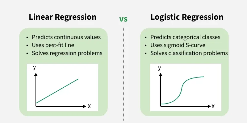
Differences Between Linear and Logistic Regression

Logistic regression and linear regression differ in their application and output. Here's a comparison:

Aspect	Linear Regression	Logistic Regression
Definition	Linear regression is used to predict the continuous dependent variable using a given set of independent variables.	Logistic regression is used to predict the categorical dependent variable using a given set of independent variables.
Problem Type	It is used for solving regression problem.	It is used for solving classification problems.
Output Type	In this we predict the value of continuous variables.	In this we predict values of categorical variables.
Curve/Model Fitting	In this we find best fit line.	In this we find S-Curve.
Estimation Method	Least square estimation method is used for estimation of accuracy.	Maximum likelihood estimation method is used for estimation of accuracy.
Output Example	The output must be continuous value such as price, age etc.	Output must be categorical value such as 0 or 1, Yes or No, etc.
Relationship Requirement	It required linear relationship between dependent and independent variables.	It not required linear relationship.
Collinearity	There may be collinearity between the independent variables.	There should be little to no collinearity between independent variables.

Topics

Monday, 12 January 2026